Supervised learning
Predict output according to the correct dataset which are already known.
Supervised learning problems are categorized into “regression” and “classification” problems
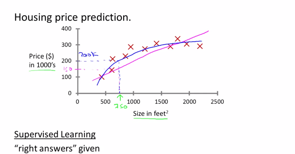
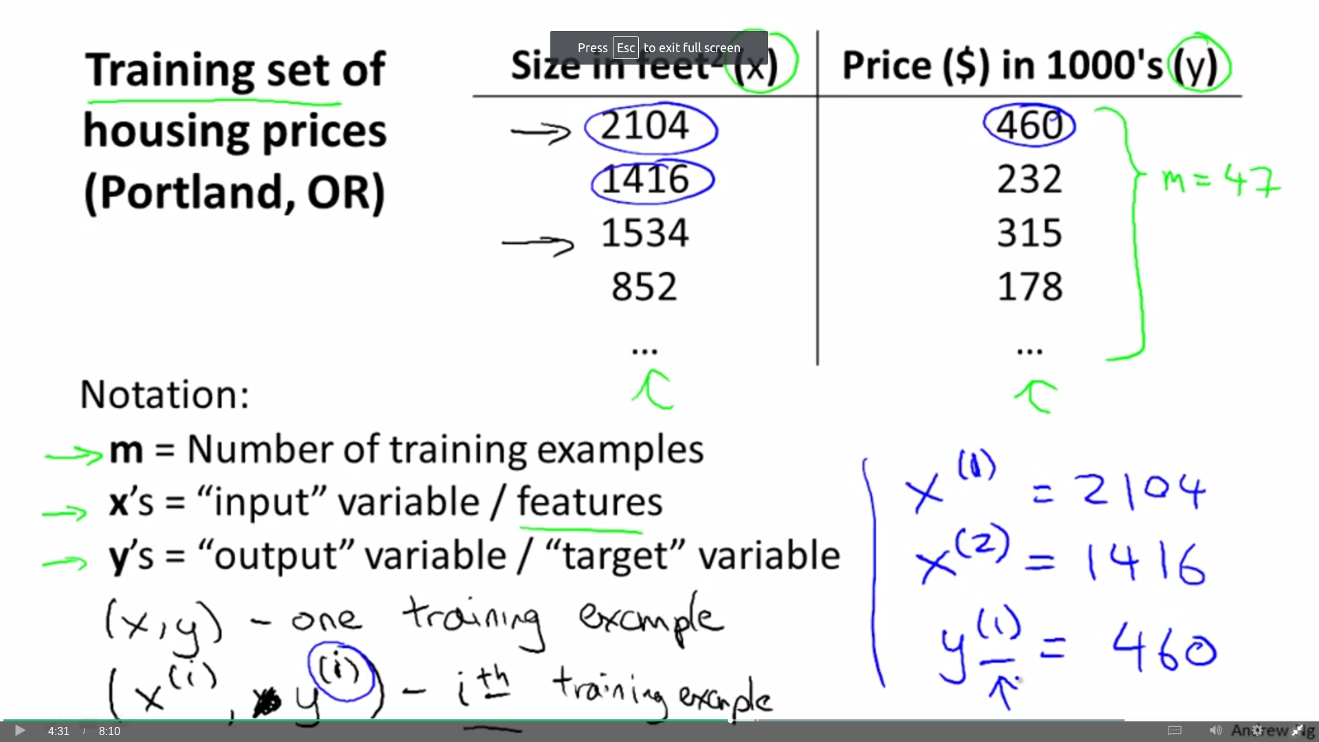
House price prediction
This is a regression problem, whose prediction value is continuous.
Do regression according to history data, you can do linear regression or quadratic regression which is up to you.
Then do prediction using this result.
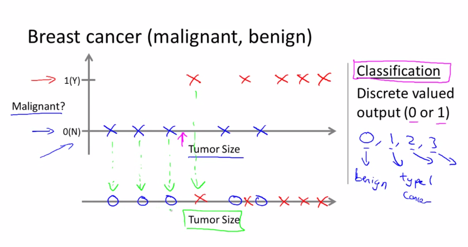
Breast cancer
This is a classification problem, whose prediction value is discrete.
Predict if tumor is benign or malignant according to tumor size. This is a classification problem.
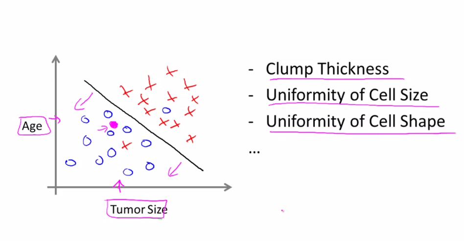
When there are two feature: tumor size and age, it will be like this:
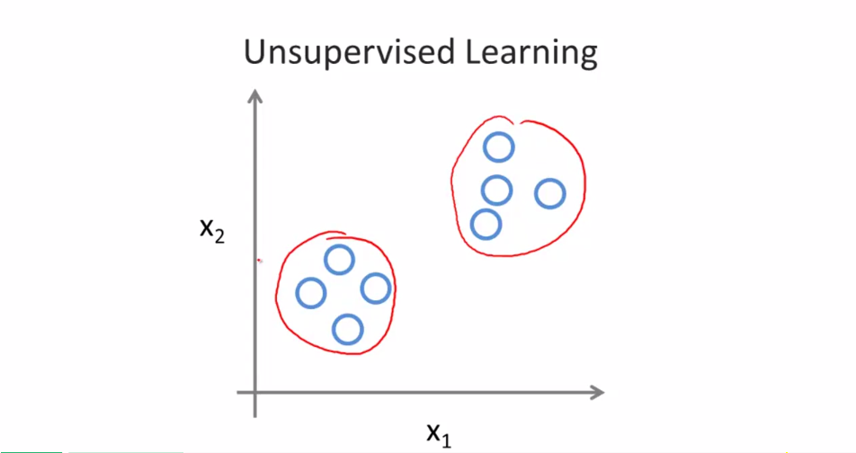
Unsupervised learning
Find data structure from given dataset which do not have right answer.
Clustering problem
Cluster these data into two parts.
An application: google news will cluster different news from different site but with same topic together.

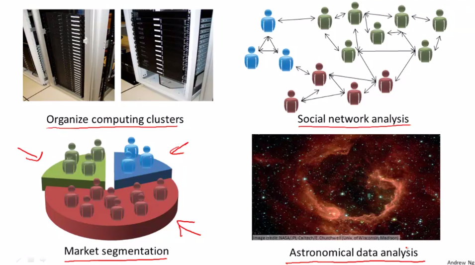
Application of Unsupervised learning.
- Cluster the servers to make it more efficient
- Cluster the user in social network
- Market segmentation
- Astronomical data analysis
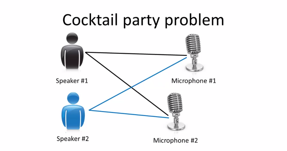
Cocktail party: Identify the voice from a mesh of sounds in chaotic environment.
Model and Cost Function
Notation
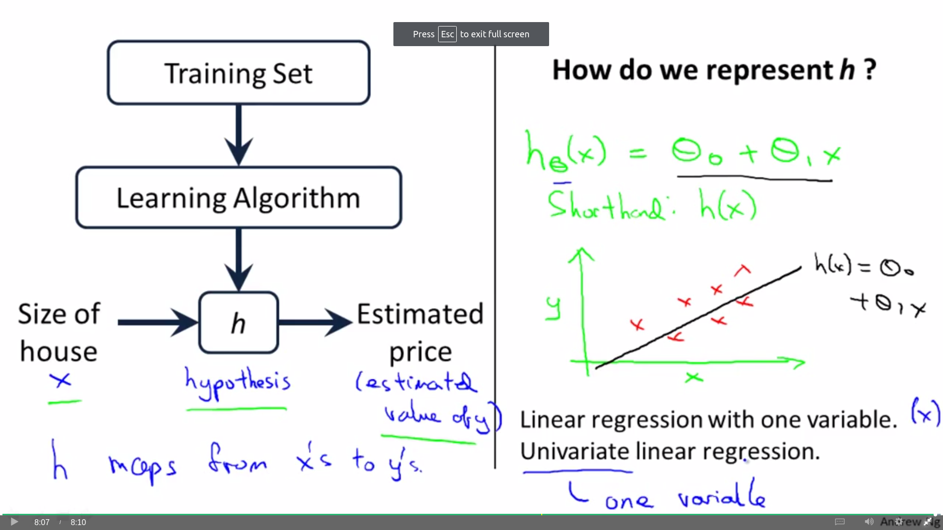
Model
why use hypothesis to represent function h: Former research used it, maybe it is not the best choice, but it just a terminology.
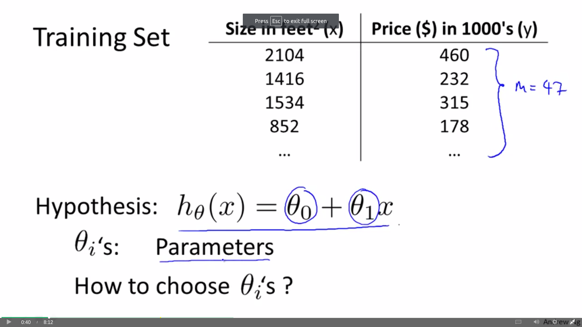
Cost Function
theta 1 and theta 0 are parameters of function h.
Something I don’t know before:
#: hash sign, represent the number of something.
1/m: 1 over | the 2m
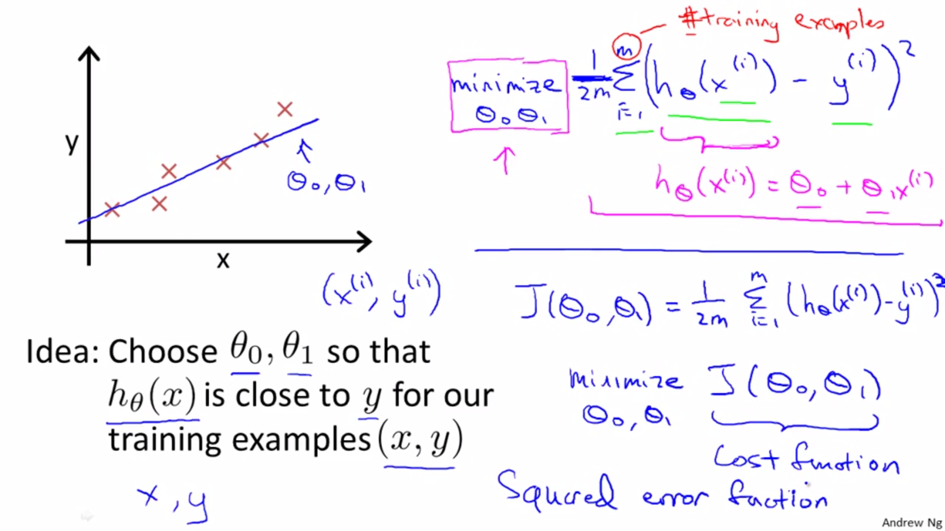
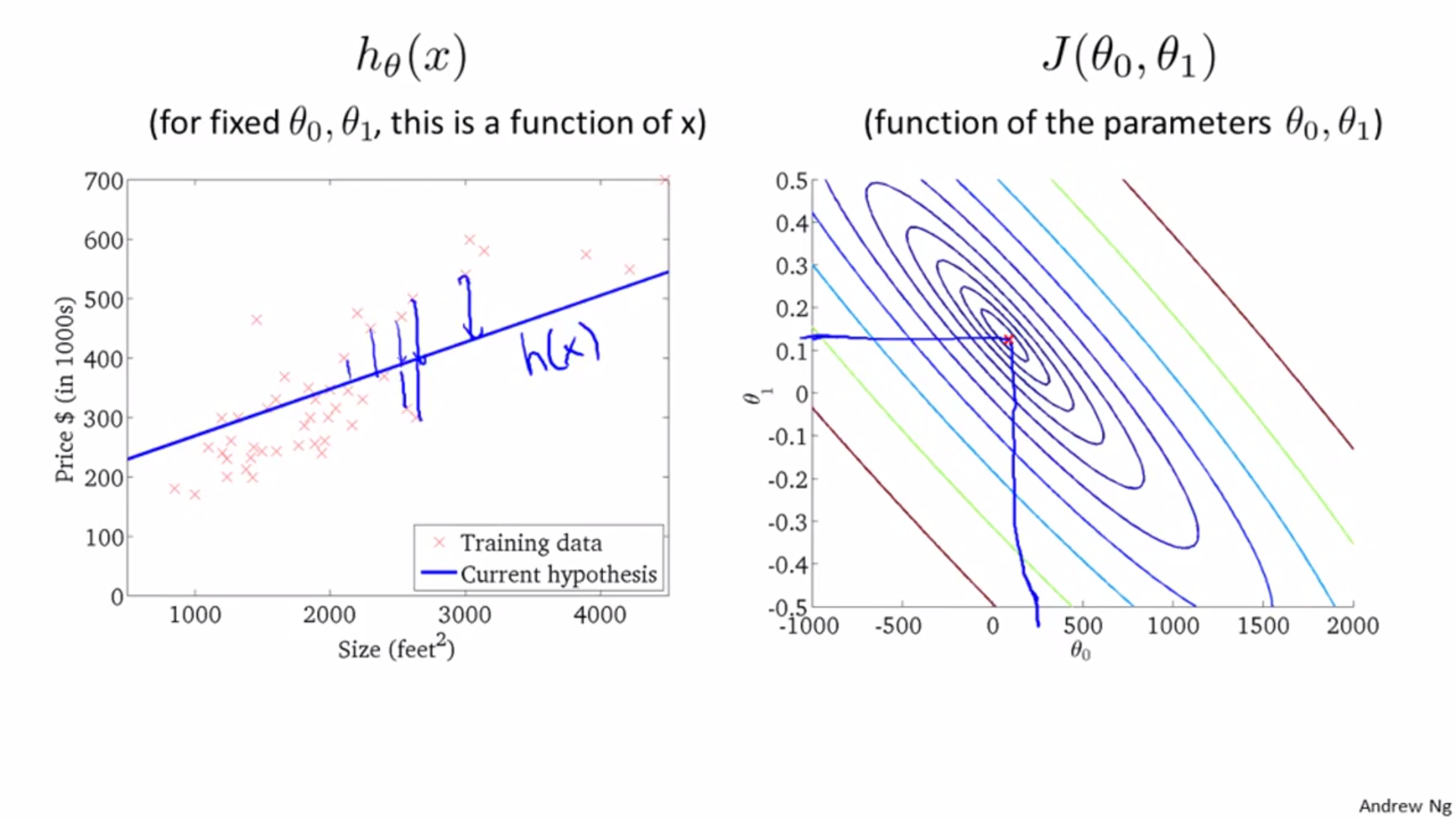
The figure as follow shows the detail of cost function J of linear regression function, which can be call squared error function.
The mean is halved (1/2m) as a convenience for the computation of the gradient descent, as the derivative term of the square function will cancel out the 12 term
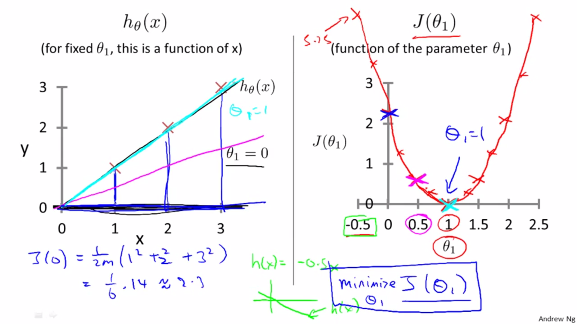
Intuition of cost function:
One parameter:
Two parameters:
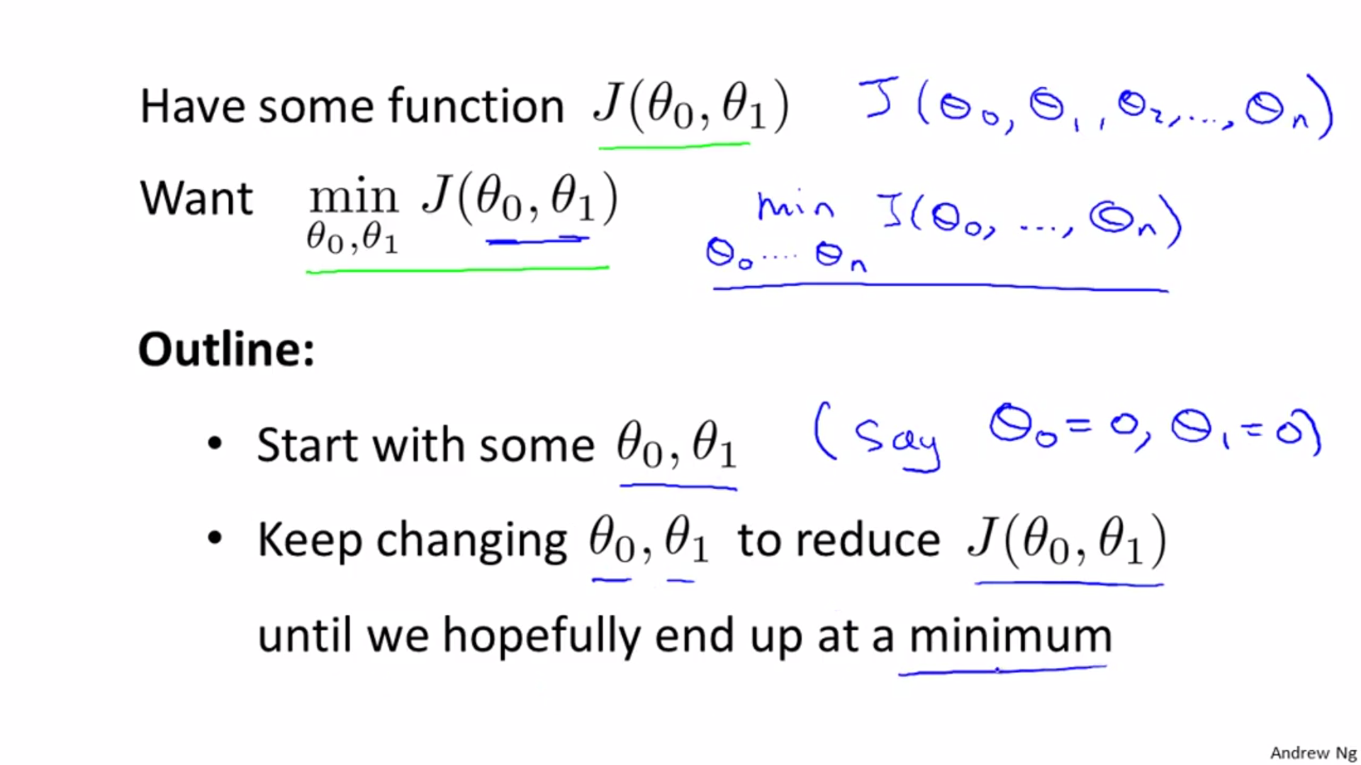
Parameter learning
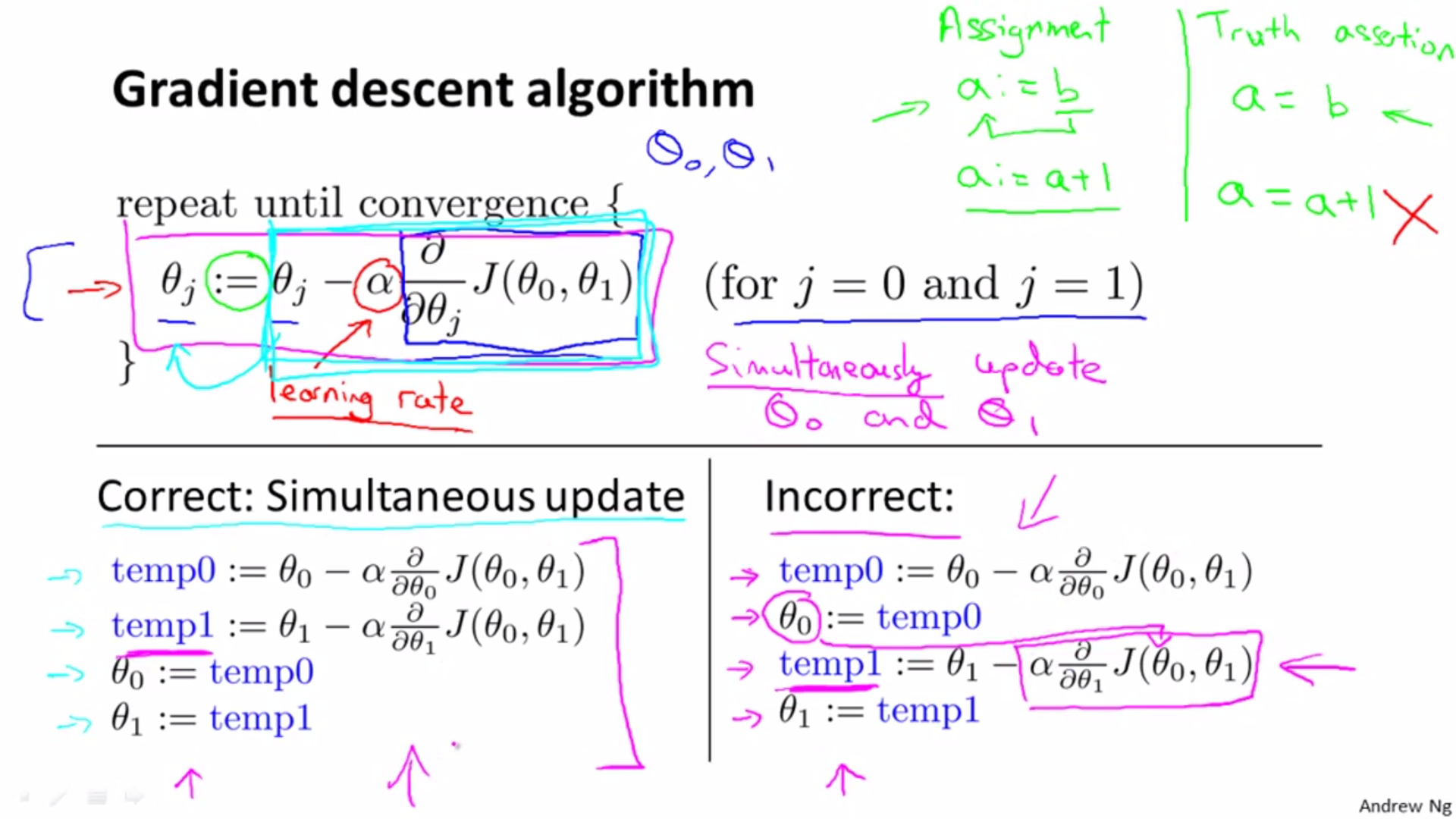
Gradient Descent
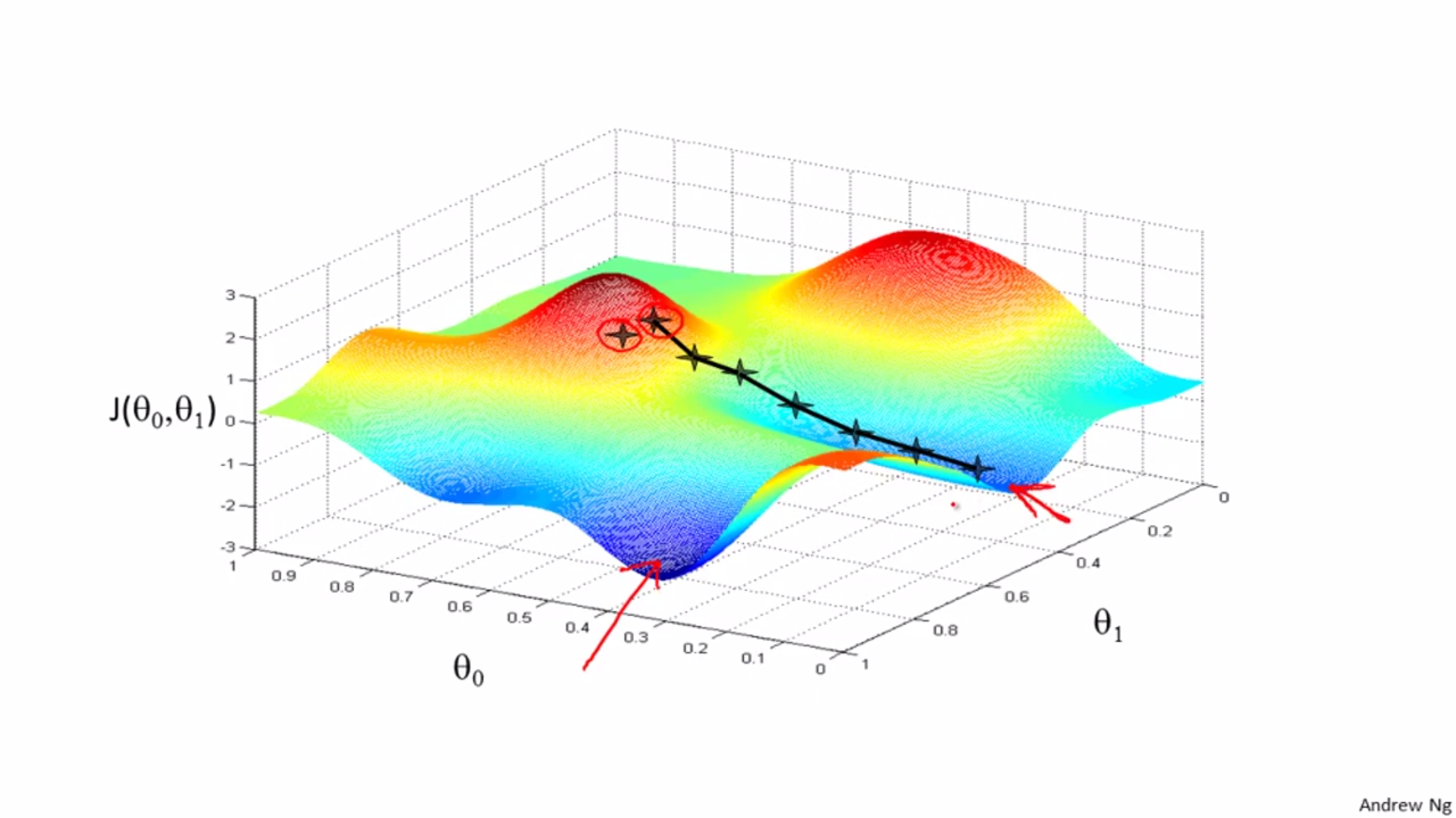
Init theta 0 and theta 1, change these two values till J reaches local minimum value.
Different start position can lead to different local optimal.
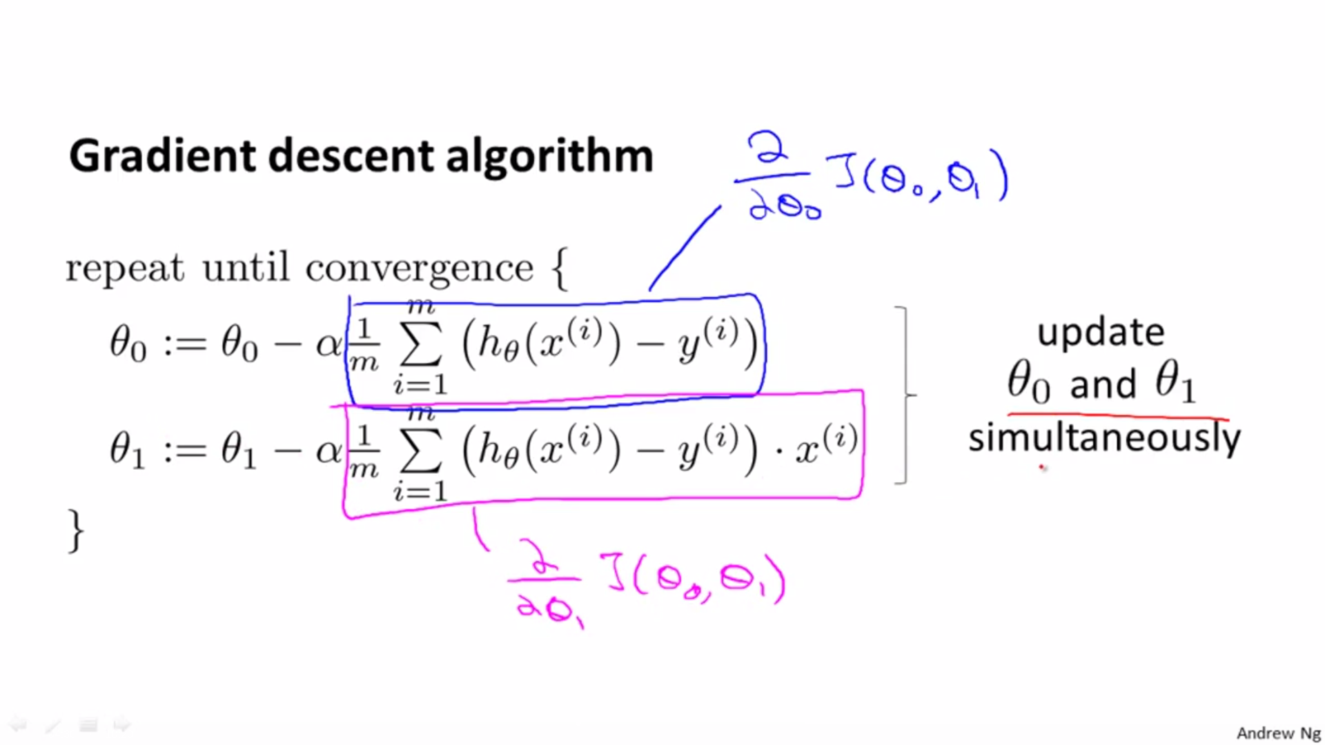
:= is assignment; = is truth assertion.
Right side of equation should be updated simultaneously.
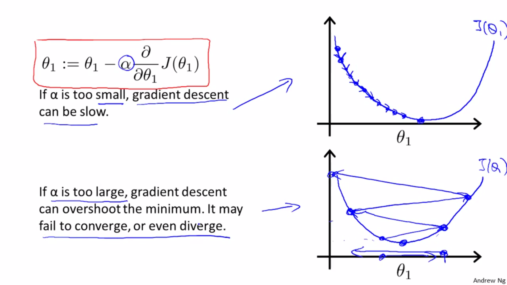
Gradient Descent Intuition
Case of one parameter:
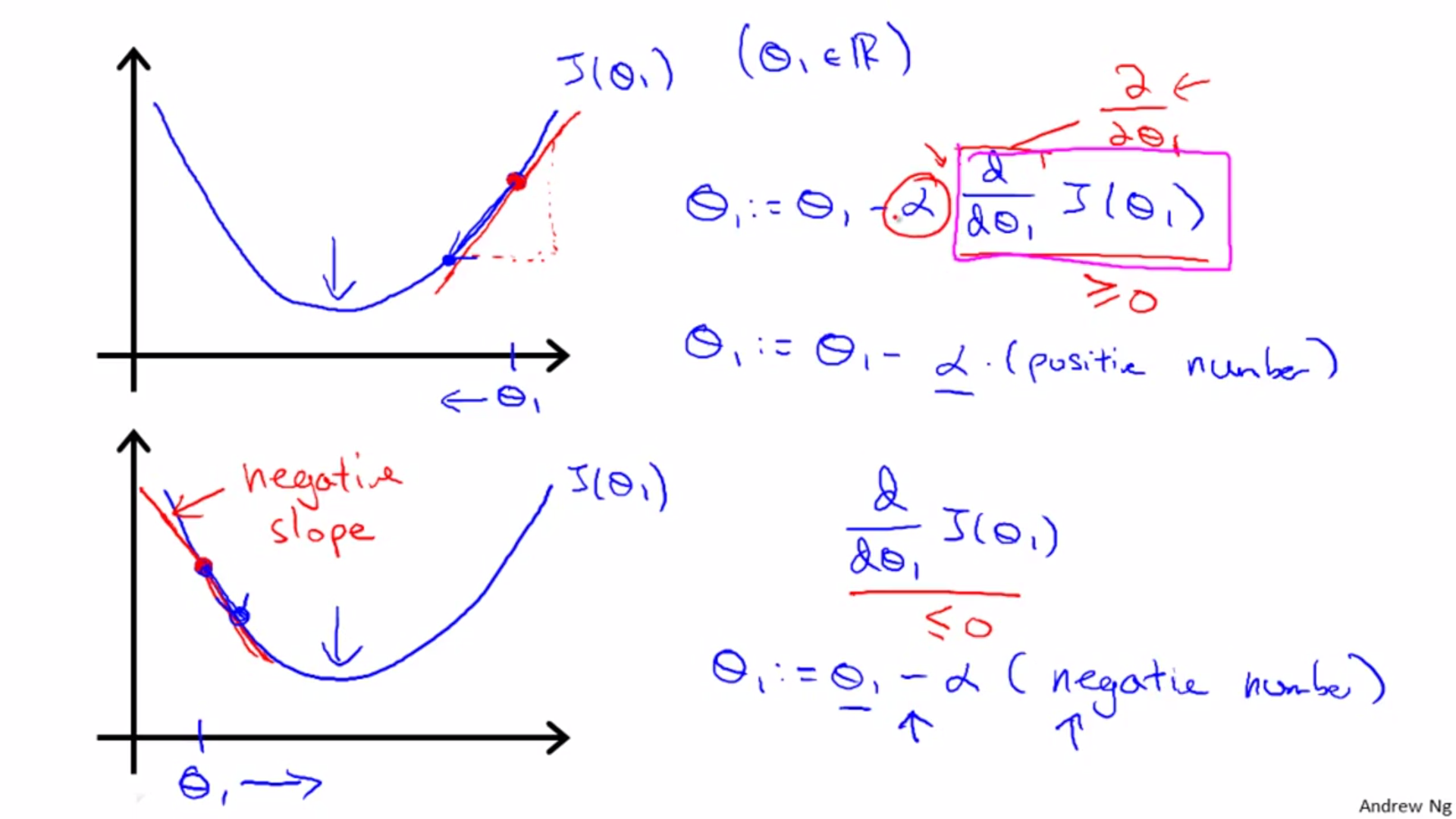
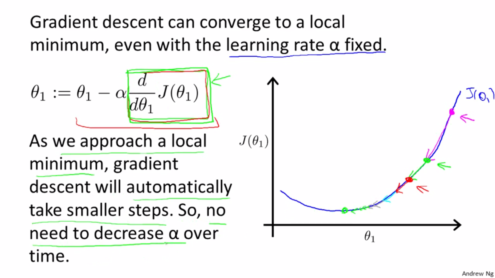
The step will be smaller and smaller, so there is no need to decrease alpha.
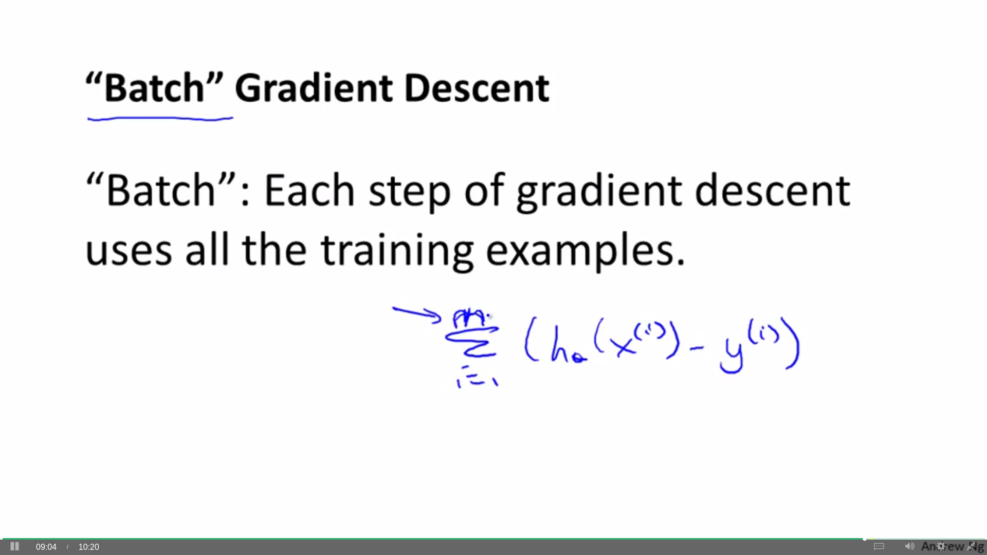
Gradient Descent for Linear Regression
Calculate partial derivation of J:
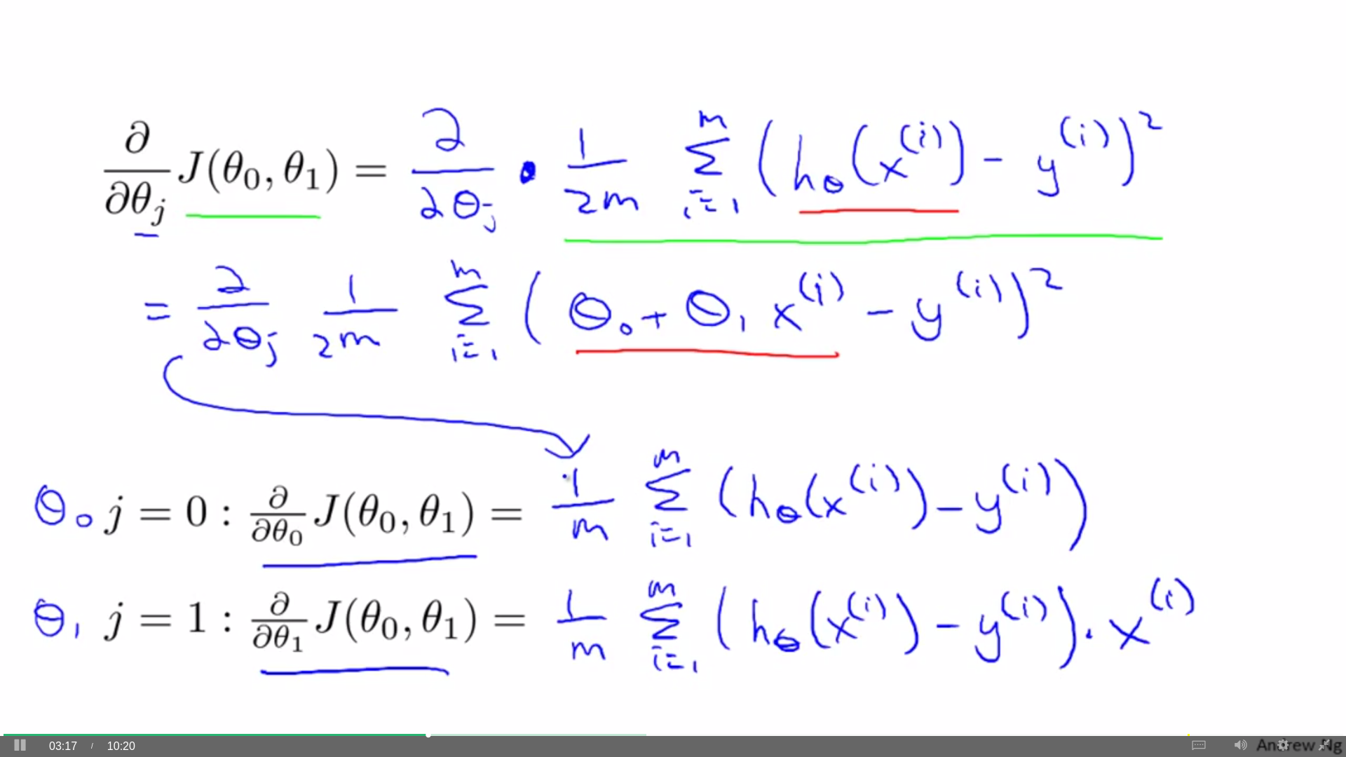
Gradient descent algorithm for linear regression:
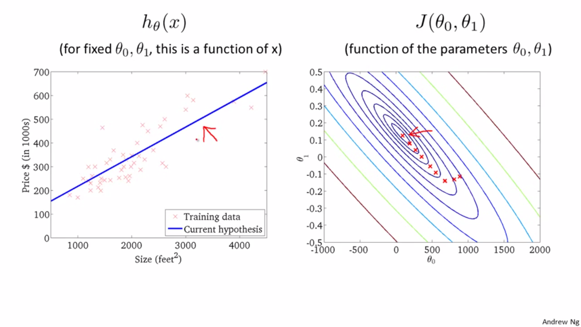
Process of descent for linear regression
Batch gradient descent: calculate all data in every update, high cost: